
Wifi Time
31 May 2026Progress: Abandoned
It's another obsessive post about timekeeping!
Here I'll describe an abandoned project to build a "fake" GPS module that grabs the time over WiFi, to function as a drop-in replacement for the GPS breakout boards used on earlier versions of my Precision Clock. My mistake was being too ambitious, the almost impossible goal of getting sub-millisecond accuracy, over WiFi, using regular NTP at slow polling intervals, and with only the built-in oscillator of an ESP8266. It perpetually felt like I was on the cusp of accomplishment, and in the end I petered out without posting anything.
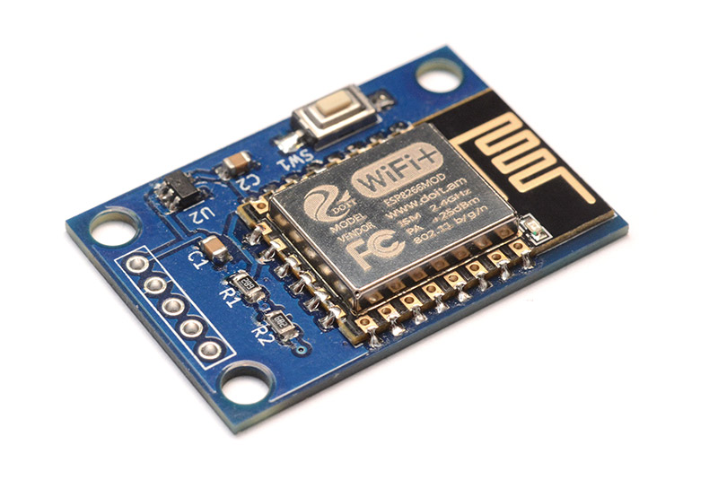
It's been about six years since I last touched this, and given that the Mk IV clock has a much better GPS module (along with an SMA connector for a better, or better placed, antenna), it's unlikely I'll ever finish it. But the other day as I wrote up my virtual precision clock with its comical NTP proxy I was reminded of these earlier experiments, and thought they might be worth sharing.
I'll now briefly hand the narrative over to my younger self, for the partial writeup I did in July 2020.
NTP Precision Clock Module
If you're looking to build a precision clock, look no further than GPS. Nothing gives you such excellent results for so little effort. Even the cheapest GPS modules have timing accuracy in the tens of nanoseconds.
But indoors, GPS reception isn't great. Especially in new homes built with aluminium-lined insulation, sometimes a GPS signal simply isn't reliable.
NTP, the Network Time Protocol, is several orders of magnitude less accurate than a GPS module, but in many buildings it's easier to pick up a WiFi signal than GPS.
I have no interest in building a WiFi-enabled Precision Clock. The idea of connecting it to the internet turns it into a different type of clock. The next version of my Precision Clock is unlikely to feature WiFi. But... there is a certain appeal to a "fake GPS" module, which can be dropped into the precision clock, to convert it to a WiFi NTP clock.
There's an existing project that does exactly this. An ESP8266 is used and it outputs NMEA strings just like a real GPS module. I took a look at it and it's a pretty good attempt, but there are few reasons it's not sufficient for a Precision Clock.
- The time calculation is inaccurate. It's roughly correct, but well outside of the millisecond tolerance I'm aiming for.
- The PPS signal is treated carelessly, such as toggling it while waiting for WiFi to establish. The PPS signal should only be pulsed if the time is accurate.
- There are a bunch of other signals emulated, and a serial interface, all of which we don't care about. On the other hand, we don't want the WiFi credentials to be hard-coded, so a soft-AP interface would be good.
Environment
The example I linked to above is built using the Arduino environment, with the ESP8266 "core". I installed this to try it out, and I must say, although I hate many aspects of it (the bloat, and how it glosses over important details) it's hard to argue with the ease of getting started. The last (and only other) time I attempted a project with the ESP8266 I installed the SDK and toolchain manually, and it took bloody ages.Although I'm starting over, I decided to continue with the Arduino environment if possible.
There are dozens of NTP implementations for Arduino and ESP8266, but looking at their code is disheartening. The included "NTP library" performs the time measurement by calling delay(10) in a loop and counting the iterations. So even if the rest of it was perfect, the result would be, at best, quantized to 10ms increments. I have to be realistic about the level of precision we can achieve – a few milliseconds is probably the best we can do – but we might as well implement the standard correctly, and to the best of our timing ability.
Another problem with beginner-friendly environments is that many of the tutorials and examples are produced by blindly copying and pasting code chunks from each other. The example NTP implementation inexplicably fills out some of the NTP header with junk, and many other examples and implementations have copied this exact code, without explanation.
In fact, you only need one single byte to be non-zero to form a working NTP request. The first byte needs to indicate that we're a client, and optionally the NTP version. The remainder of the 48 bytes can be left zero, they'll get filled out by the server.
NTP stamps
There are many guides on the internet explaining the operation of NTP.In essence, we send a request and wait for its response, measuring the time taken. The response has a couple of timestamps set by the server. We add half the time taken for the request to return and we've got ourselves an accurate timestamp. If the network route is symmetrical, this should be accurate to well within a millisecond.
NTP timestamps are 8 bytes. The first 4 bytes are the number of seconds since January 1, 1900. Very similar to the unix timestamp, except tediously different. It's an unsigned number, so it will overflow in 2036, two years before the unix timestamp rolls over.
The next 4 bytes are a fractional offset, so the full 8 bytes makes a fixed-point number.
The example NTP code manually turns this into a date and time string, but the standard time.h stuff is already included by default, so all we need to do is add an offset to get the unix timestamp, and call gmtime and strftime.
Endianness
The timestamps in the NTP packet are in network-byte-order, i.e. big endian. The ESP8266 is little endian by default (the processor can technically support both, but I doubt it's possible to switch within the Arduino environment).
I gladly bid goodbye to endless shifts for switching between byte orders when I found out about a relatively new feature of gcc: scalar_storage_order("big-endian") Adding this attribute to a struct will enforce that endianness, regardless of platform. Any shift instructions needed will be generated automatically.
Sadly, this didn't work at all here. Arduino is C++, not C, and g++ does not support this extension. Worse than that, by default all warnings are suppressed, so it doesn't even tell you that it's ignoring the attribute.
We now return to your regular writer in this the year 2026, where I'll do my best to remember the juicy details.
Pulse Measurement
The most important part is being able to measure our output. We're lucky enough to have the real GPS module to hand, and at the tolerances we're working, its PPS output can be considered gospel. The main thing is to stick a really good antenna on it, so it doesn't lose its fix.
We will create our own PPS output on the ESP8266, which can then be compared to the GPS output, and the best tool to do this is a logic analyser. Luckily I had invested in this, the world's cheapest logic analyser:
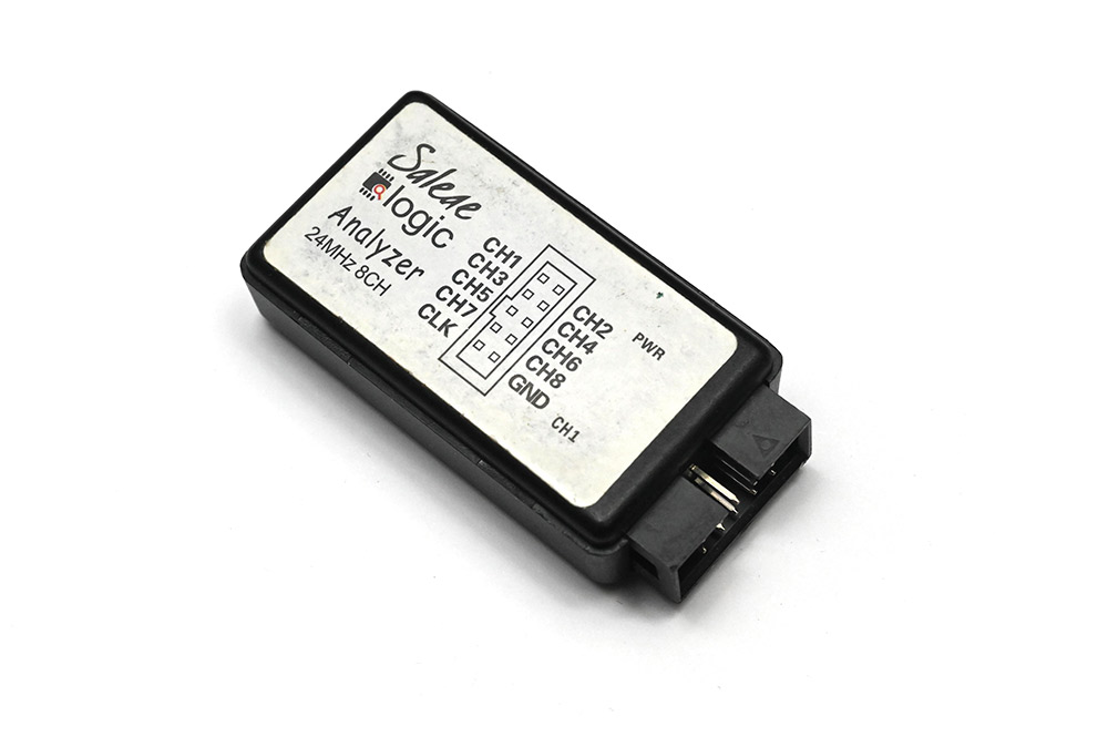
This 8 channel, 24MHz USB logic analyser cost about £5, and they had the audacity to write "Saleae" on it, along with some delightful Comic Sans. But it's more than adequate for what we need to do.
The chipset on the device is a Cypress FX2, and the interesting thing is that the firmware is loaded into RAM on powerup over USB. The open source fx2lafw firmware can be loaded by sigrok for us.
We want to sample at the highest resolution, but over a period of many minutes, potentially hours, which would be a huge amount of data. Much better would be to store just the offsets between the two pulses each second. Sigrok supports many protocol decoders, and I understand it's not too difficult to write your own, but an existing decoder called "Jitter" is able to do everything we need. We instruct it to consider the GPS PPS as clock, and our ESP8266 PPS as the signal.
The command was something like this:
sigrok-cli -d fx2lafw --config samplerate=200kHz --samples 800M -C D0,D1,D2,D3,D4 -P jitter:clk=D0:sig=D4 -B jitter
This could be piped (or tee'd) into a file giving us a list of offsets, which could be pasted into a spreadsheet. A command-line alternative is gnuplot, which is ancient and quirky, but as I was repeating this dozens of times it made sense to get this automated. Apparently, at the time I was going through a perl phase, as I made a tiny script that sat between them like this:
#!/usr/bin/perl

$| = 1;

while (<>) {
  chomp;
  print $i++ . "\t";
  while ($_ > 0.5) {$_ -= 1.0;}
  print $_ . "\n";
}
This also compensates if the jitter amount has wrapped by a whole second, which would sometimes happen if we started it at exactly the wrong moment. In order to watch the graph in real time, my gnuplot file looked like this (optionally fix yrange as needed):
plot "plot.dat" using 1:2 with lines
#set yrange [0:0.004]
pause 1
reread
I wish I had made more detailed notes at the time, but obviously my focus was on getting the pulse timing right, rather than on documenting how the graphs were plotted. I remember that my eventual setup was a single command, that would start logging the offsets, and also plot them in real time, which made the development slightly less painful than it otherwise would have been. It still involved waiting for ~15 minutes to see the effects of any changes we made though.
Hardware setup
Experiments were carried out on this rather grotty old breadboard. I'll suggest it was a bit cleaner at the time, and accumulated grot during its subsequent storage.
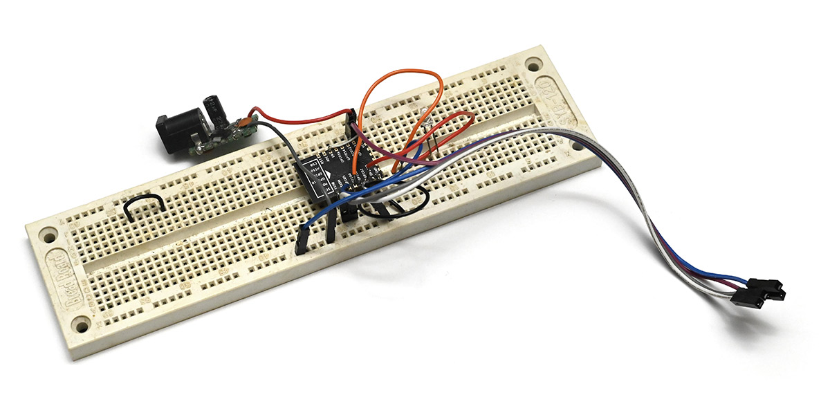
The flying barrel jack has a regulator on it. Not shown are the FTDI cable for reprogramming, the GPS module for comparison, and the logic analyser.
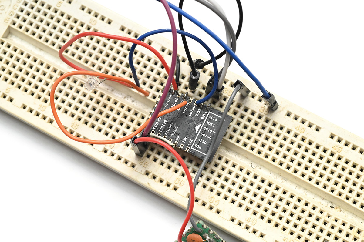
I did also produce a prototype on protoboard, but this was less useful for developing and measuring its performance.
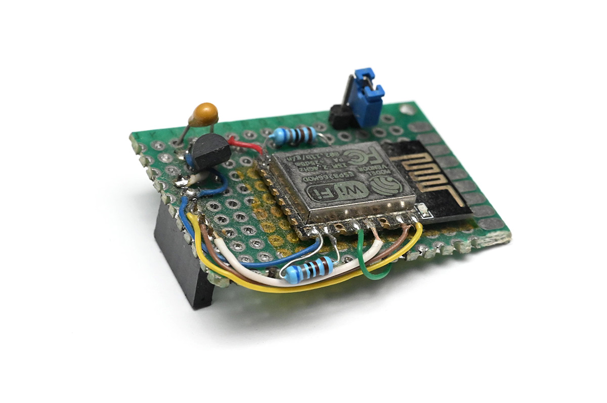
The jumper is to put it into programming mode, which conveniently uses the same TX/RX pins as the NMEA.
Discipline and NTP Etiquette
Polling NTP gives us an instantaneous estimate of the time. It assumes the round-trip is roughly symmetrical.Due to the terrible unpredictability of WiFi, we'll need to make lots of estimates to average out the jitter. Packets can have a random delay added in either or both directions.
Once we have some estimates, we need to discipline our own oscillator, so that we can keep time between polls. I have often wondered what the etiquette is for NTP, as it's an unauthenticated UDP packet, and how frequently you'd have to poll this free service to be considered a nuisance. Default NTP installs rarely poll faster than once every 64 seconds, and often they only poll once an hour, or every few hours. I worry especially when I'm producing a circuit board that I (at the time) planned to distribute to others, even if only in small numbers.
My general plan was to start off polling every 16 seconds, and then gradually back off as the estimates agreed with one another.
The onboard oscillator of an ESP8266 is not particularly accurate. Disciplining it is more complicated than simply polling, seeing if we're fast or slow, and adjusting it. To eliminate outliers, to average correctly and hopefully backoff with the polling, we need to keep a history of estimates and adjustments, but those timings are referenced to an oscillator that's now changing. It is quite a complex control loop problem.
Instead of disciplining the main oscillator, we can pretend it's stable and discipline a secondary timer derived from it. The main oscillator will still drift with temperature, but hopefully slow enough that it doesn't play havok with our estimates.
First Plots
Perhaps the story is better told through graphs. The very first capture looked like this:
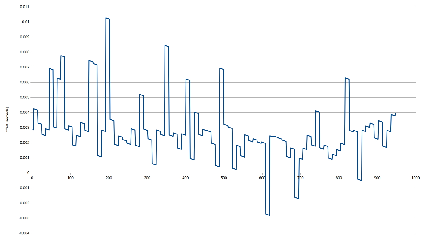
In this and subsequent plots, the horizontal axis is in seconds, where 1000 is about 16 minutes. The vertical axis is also in seconds, showing the offset between the PPS pulses. In this first plot, we simply polled NTP every 10 seconds and attempted to output PPS accordingly.
It's immediately obvious that there are plenty of outliers, with a bias towards the positive. The flat where I lived at the time had atrocious WiFi contention, with dozens of overlapping networks. I'm not too familiar with the physical layer of WiFi, but maybe the chances of a packet collision are greater in one direction than the other. If the initial outbound packet is unable to be sent because the channel is busy, it will be delayed, but once the channel becomes free it (possibly) remains free for the next second or so, meaning a collision is less likely on the return. I'm just speculating though.
Measured again, some of the outliers were more than 15ms.
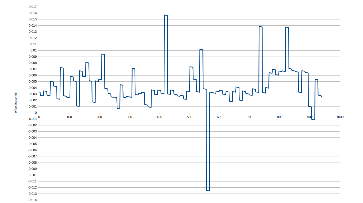
Aside from the outliers, the average seems to be settling somewhere around 3 milliseconds off, which was a puzzle at this point.
Eliminating the outliers by keeping track of our estimates and discarding results that cross a threshold, our results are still pretty unsatisfactory:
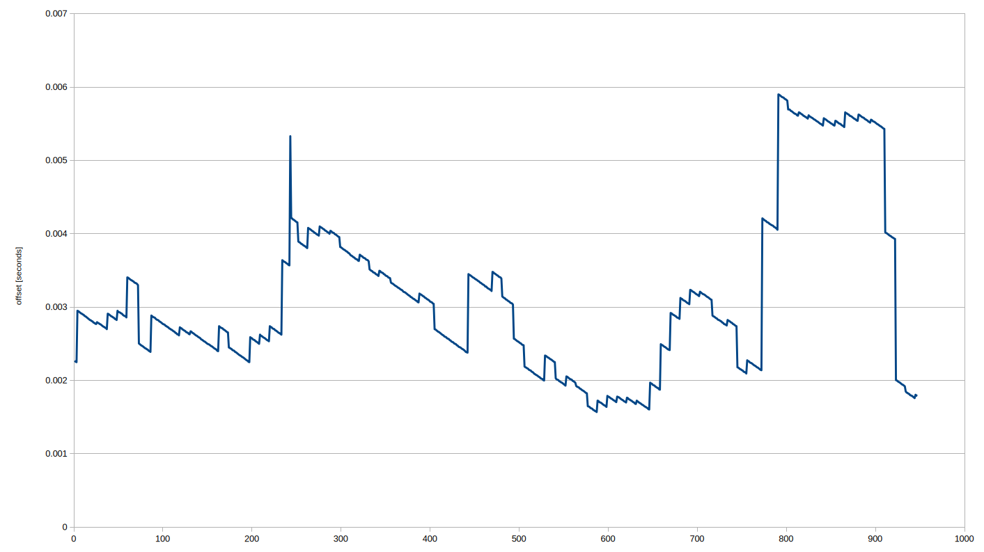
Note the vertical scale has changed. The slope of the lines between polls is the same as before, just more visible. It represents the drift of our uncalibrated oscillator, which we are not yet disciplining.
Many acquisitions later, I was sometimes getting plots as good as this:
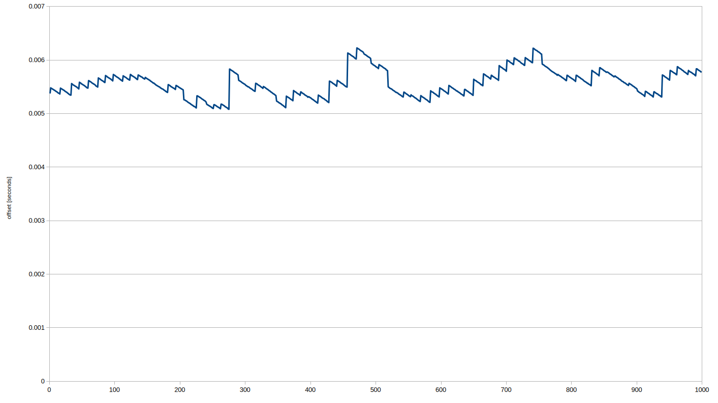
Even undisciplined, the results agree almost within a millisecond, which is fantastic. The systematic offset remained a mystery for the moment. Have a think what it might be...
Loop tuning
If our oscillator discipline works well, the slope of the line between each poll should flatten to be perfectly horizontal. Then we can back off on the polling and coast on our tuned oscillator.Initial attempts gave some amusing results.
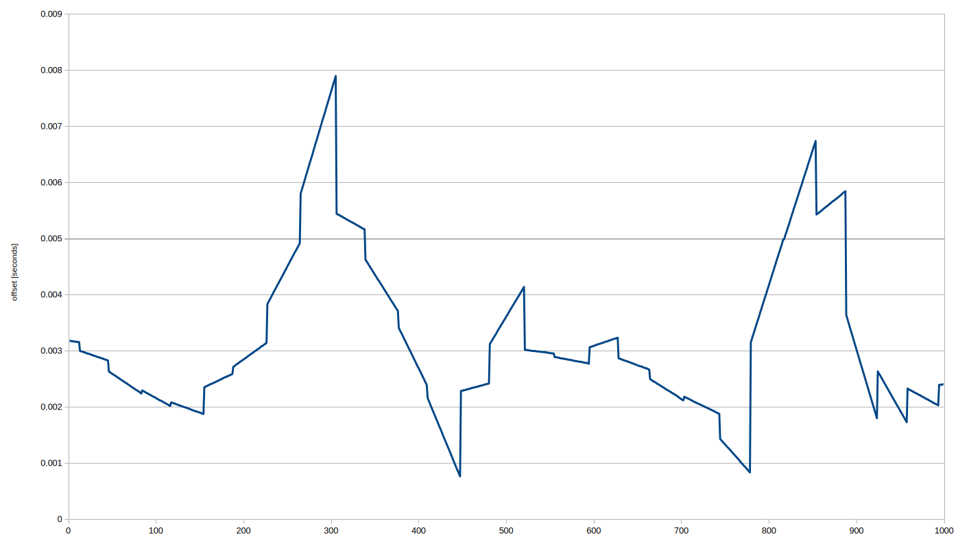
Our correction overcompensates, and the system becomes unstable. As part of our attempt to enforce stability, we average the result of each poll with previous estimates, limiting the effect of a single data point.
Fiddling with the parameters for our control loop could even, almost, be described as fun, if it didn't take another 16 minutes to check what effect it had.
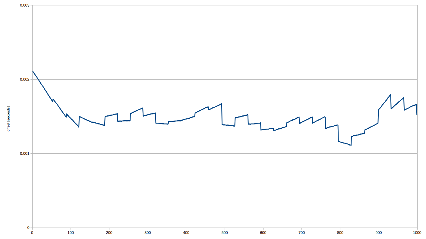
Systematic Offset and the Pool
The offsets were consistent throughout the measurement, but different if we measured again on a different day. Embarrassingly late, I finally figured out why the numbers converged a few milliseconds off: the time reported by NTP was wrong.
The NTP "pool" is a collection of servers that report the time, for free. The majority of these servers are run by volunteers. When you request pool.ntp.org (or a subdomain), it returns the IP address of a geographically nearby server that's part of the pool. Most of the servers are not "stratum-1" servers, that is, they themselves are only synchronised to other servers by NTP.
We do the DNS lookup before we start polling (it would ruin the timing otherwise) and then hold on to the server IP address for maybe a few hours or more. With some logging we can correlate performance to IP addresses, and it became clear that the results were substantially better on an occasionally returned IP, that, it turns out, belongs to cloudflare.
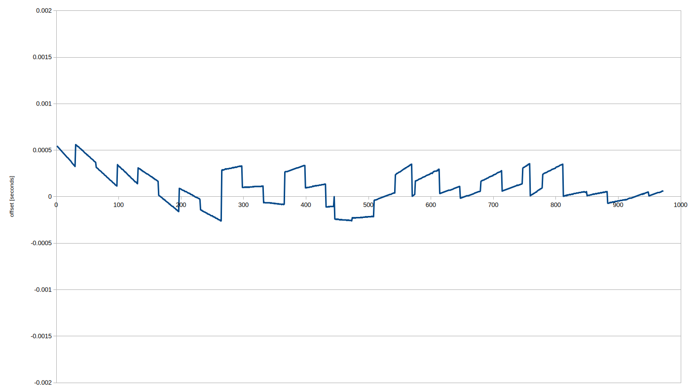
Setting time.cloudflare.com as our preferred timeserver immediately gave us a massive boost in performance. Evidently cloudflare have the budget to keep their timeservers accurate, though saying that, a standard GPS module doesn't exactly break the bank. I suppose the vast majority of people using NTP don't care about a few milliseconds.
Another environment
The second big improvement to my results came from running the experiment on a different Wifi network. Trying it at a friend's house, and at the hackspace, showed that my home network had far more jitter than most.But, it needs to run on my home network, or it's not worth bothering. At certain times of day it seemed to work a lot better, so I tried doing some longer measurements. If our control loop works well we should be able to average things out.
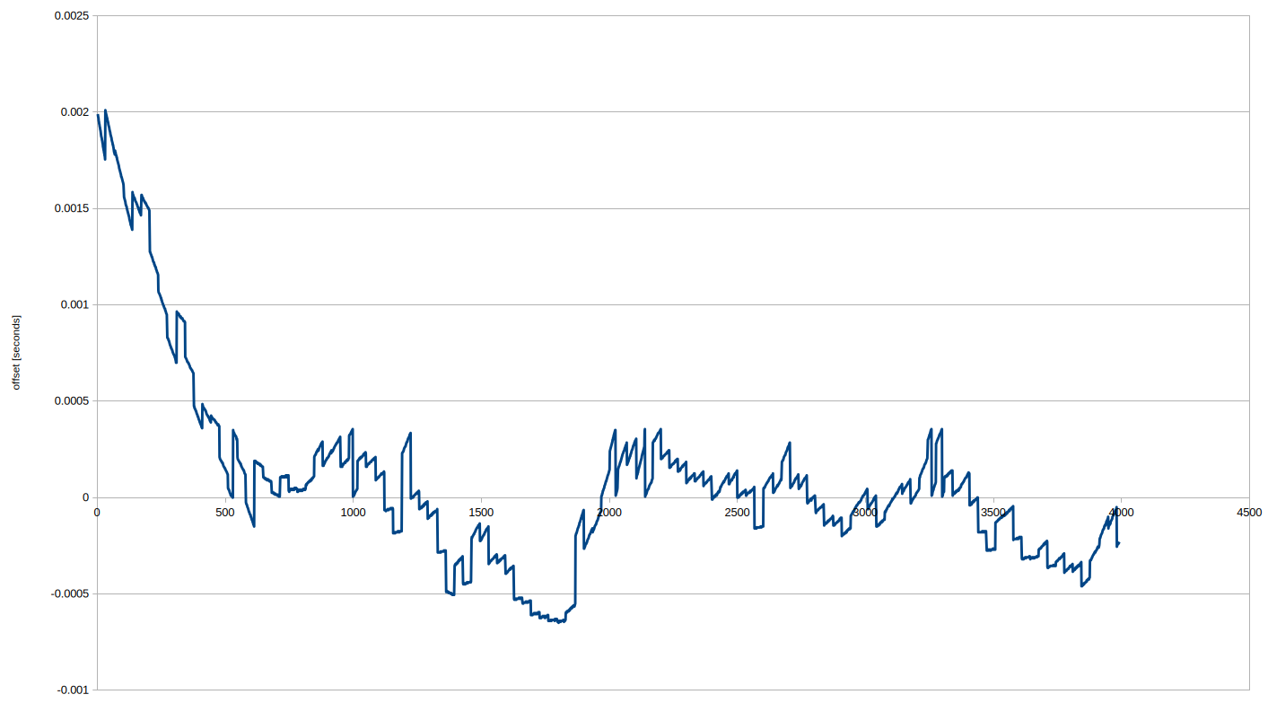
4000 points is about 66 minutes. The lead-in on the left is the powerup sequence where the oscillator is way off. On the roadmap was to maybe store our estimates in EEPROM, so that initial powerup could be a little closer to the mark.
The slope is exaggerated because the horizontal scale has changed, but really this is a fantastic result and gave me confidence that the goal was in sight. Most of that graph above is within half a millisecond of the GPS reference. All we need to do is get the control loop right, so we can back off with the polling.
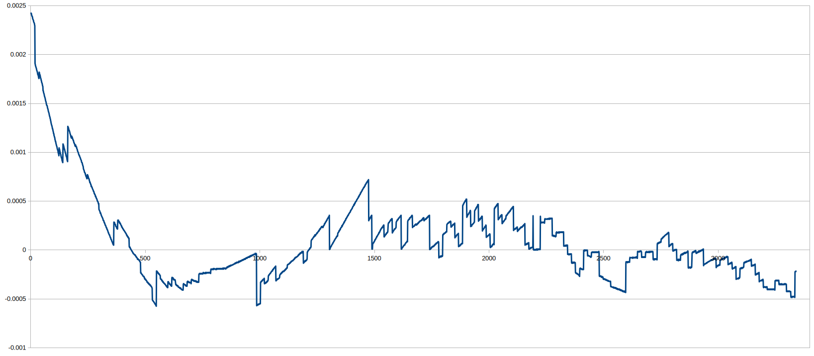
It's easy to look at these graphs and get a feel for what the loop should actually be doing, but remember, we're plotting these against a known good PPS reference. The control loop is running blind. After the undershoot, a bunch of readings seem to agree with the slope, so it backs off with the polling, and creates that peak in the middle.
I have a huge amount of plots, tens of hours of experiments, many of which involved a tiny tweak to the loop behaviour, then we wait to see what effect it had. Here's one where it oscillated wildly:
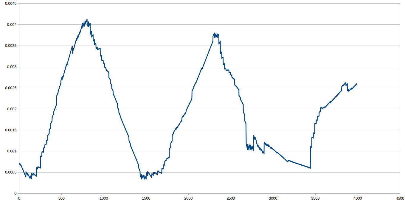
The fact that it's giving a lovely sinewave (with a period of about 20 minutes) suggests that if we could just get our averaging/damping right, we'd be onto a winner. It would take a bloody long time though. Often the loop appeared to be working well, but then after a couple of hours would start to go haywire. Here's a capture that started off OK, got a bit shaky, and by the third hour decided to run away:
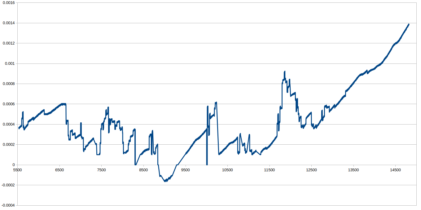
In the following plot, captured at a friend's house, I must have instructed it not to start backing off until some threshold was met. Here it managed to go for 15 minutes without polling, and stay within 0.6ms throughout. But it may just have been a fluke.
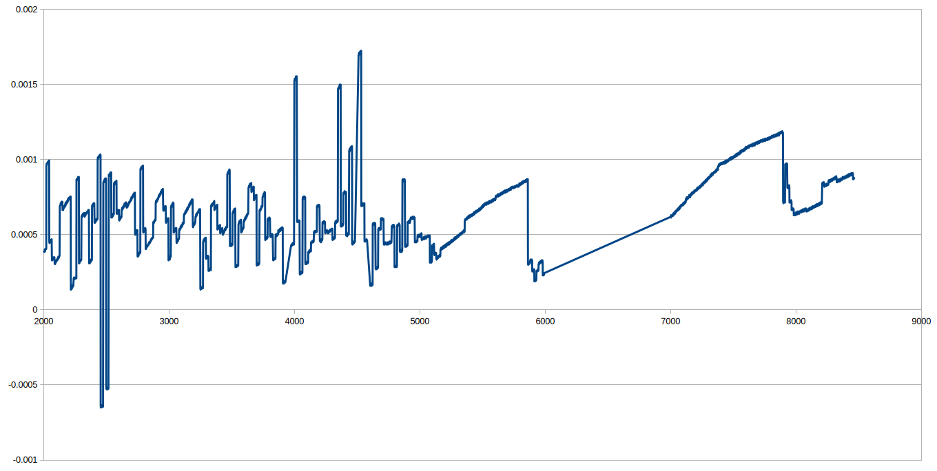
Overall, perhaps this conveys why I was never quite satisfied with the behaviour.
I'm fully aware that what I was trying to do was re-inventing the wheel. I am sure that control loops for synchronising clocks over jittery networks has been solved before. But more importantly, what I really should have done was just stick a TCXO on the board. Even without disciplining it, a TCXO will be within a few ppm out of the box. With that we could have simply polled, say, every five minutes and not bothered with anything else.
Saying that, it's definitely possible to make this work with no extra hardware. I think another approach to disciplining our oscillator would be to use the fact that we know the real wall-clock time with each pulse. Instead of adjusting based on the time between pulses, we could have just taken two measurements, ten minutes or even an hour apart, and counted the number of clock cycles between them. Even if the measurements were outliers that would give us a good estimate with little chance of instability. That does again assume that the oscillator is not changing with temperature.
Finally, since the Mk III clock I wanted to pair this with only displayed the time to the nearest 10ms, maybe there wasn't really any need to aim for sub-1ms accuracy. A 5ms or even 10ms tolerance would have been fine, no-one was going to use this for anything that matters.
PCB
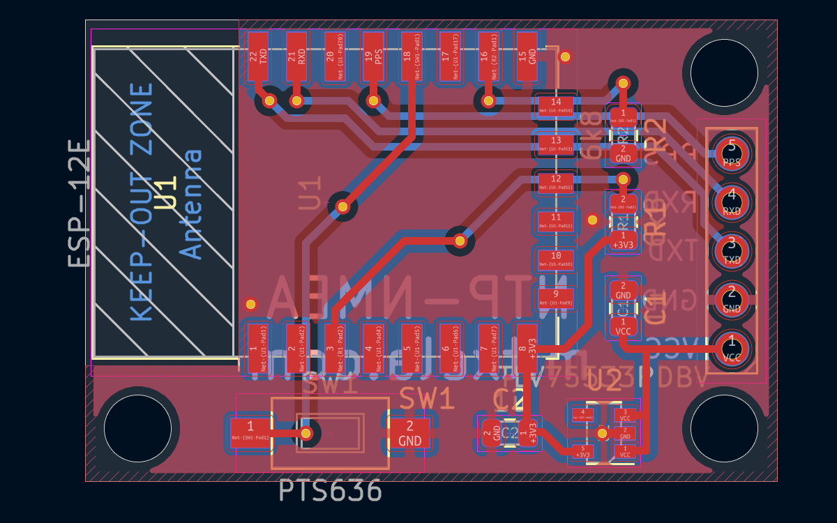
In parallel with the experiments I produced a simple PCB.
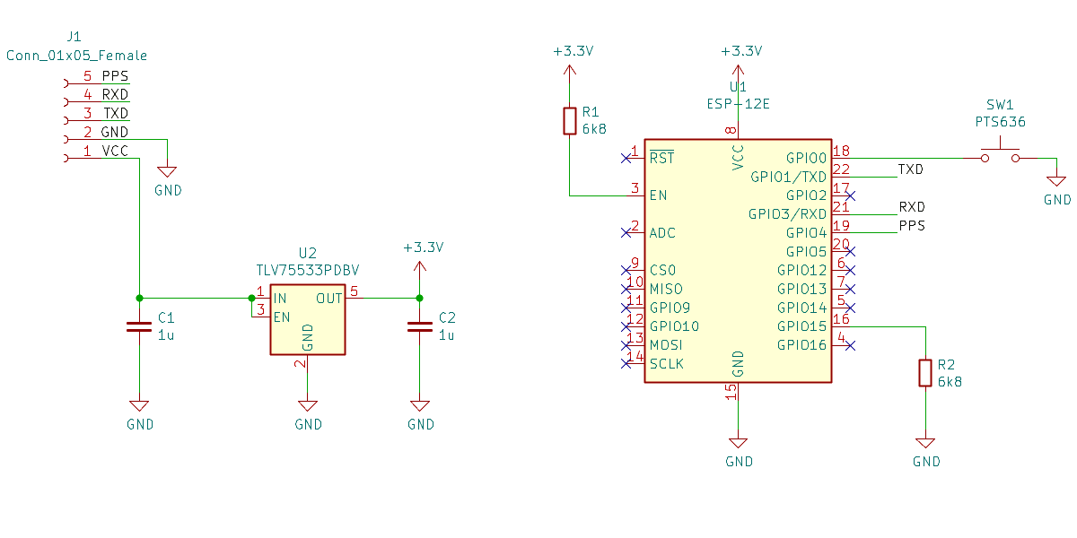
The button is both to enable re-programming, and potentially for configuration. I did set up WifiManager, which hosts an access point with a simple menu to select the WiFi network, but this normally only triggers if it can't connect. Pressing the button to begin setup would have made sense.
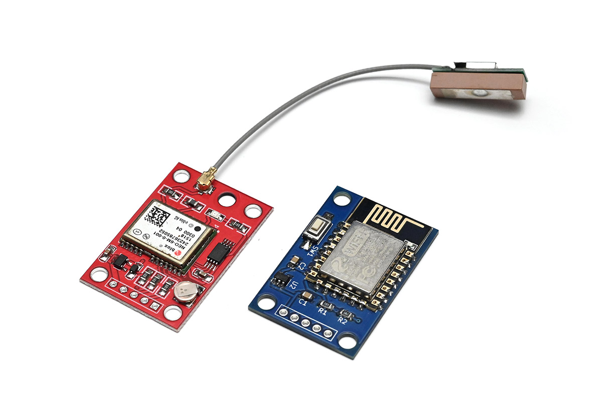
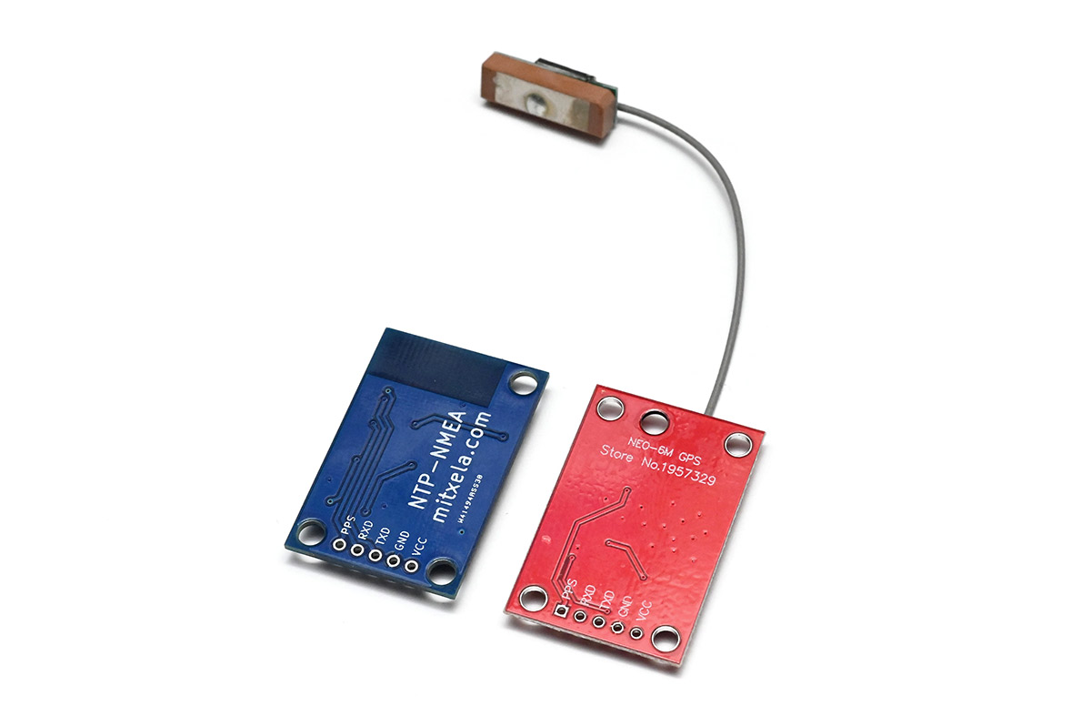
And here's the prototype alongside the GPS breakout board we were trying to imitate:
Conclusion
This project is abandoned and as such has no conclusion.I have put the source files on github. The latest commit may not be the best performing one, given what I wrote as the commit message.