Chaos Theory

11 Jan 2010
Progress: Completed

I find chaos theory fascinating, the idea that something can be both deterministic and unpredictable. What better way is there to investigate than a computer model – one with no random parameters, and input values known to a ridiculous number of decimal places. I wrote this program and write-up for an assignment in uni. Needless to say I got the highest mark possible.

Predictability of a Double Pendulum

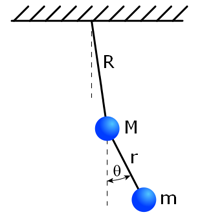
Figure 1
Double pendulum diagram
showing M, m, R, r, and θ

A simulation of a double pendulum was constructed to investigate the predictability of its final position after a set amount of time, for different initial conditions. Certain ranges were found to be predictable while others were chaotic. The boundaries of these regions showed a direct correlation to where the lower pendulum inverted.

Many natural systems exhibit chaos, such as the weather. Despite their deterministic nature these systems can be unpredictable due to their extreme sensitivity to initial conditions. Knowing what defines the chaotic regions is important in many fields.

In the simplest (Ref1) double pendulum (Figure1) m << M, thus the motion (amplitude) of M can be approximated by (eq.1).

(eq.1)

where a₀ and τ are constants of amplitude and period of M. Hence m is modelled as a single pendulum under acceleration a (eq.2&3)

(eq.2&3)

where ω is the angular velocity of m. Constants r, g are arbitrarily chosen to be 1. Initial values of ω, θ are chosen to be 0.0 and 0.1, respectively.

The first simulation evolves for t_max=100 seconds and records the θ_final. This simulation is repeated through a range of values for a₀ and τ, and plotted to a graph (Figure2). Each data-point is a shade of gray corresponding to the value of theta; it is not the brightness that is of relevance but more how it relates to adjacent points. Thus areas forming a smooth gradient represent predictable regions, while the seemingly stochastic areas correspond to chaos. Figure3 shows the same area with t_max=400 seconds. The boundary between chaos and predictability is clearer.

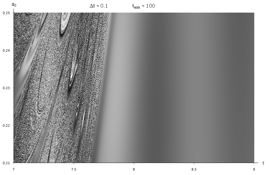
Figure 2.
Values of θ for 0.21 < a₀ < 0.25 and 7 < τ < 9 with t_max = 100

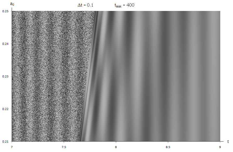
Figure 3.
Values of θ for 0.21 < a₀ < 0.25 and 7 < τ < 9 with t_max = 400

A phase-space plot (ω verses θ) for a single pendulum would be a circle. Figures 4&5 show phase-space plots for simulations inside and outside the chaotic boundary. The chaotic pendulum’s plot stretching to the left demonstrates θ leaving its normal range, i.e. it made a full rotation. Investigating this as the reason for the chaotic region, the program was modified to identify regions where the lower pendulum inverted. This was achieved by measuring the proportion of time θ escaped the range (-π,π) and highlighting the graph in red to represent it. (Figures6&7)

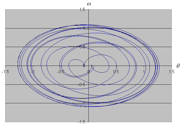
Figure 4.
Phase-space plot with a₀ = 0.251, τ = 8 and t_max = 100 The pendulum swings normally, with just a few wobbles.

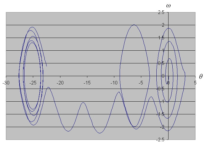
Figure 5.
Phase-space plot with a₀ = 0.251, τ = 7 and t_max = 100 The pendulum has clearly done several full inversions.

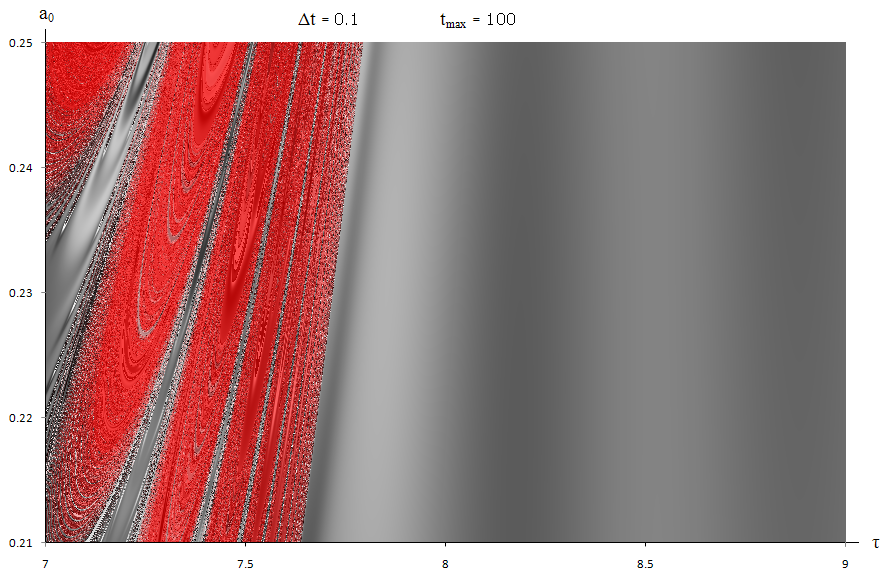
Figure 6.
Values of θ for 0.21 < a₀ < 0.25 and 7 < τ < 9 with t_max = 100 Red indicates θ went outside the region ( -π , π )

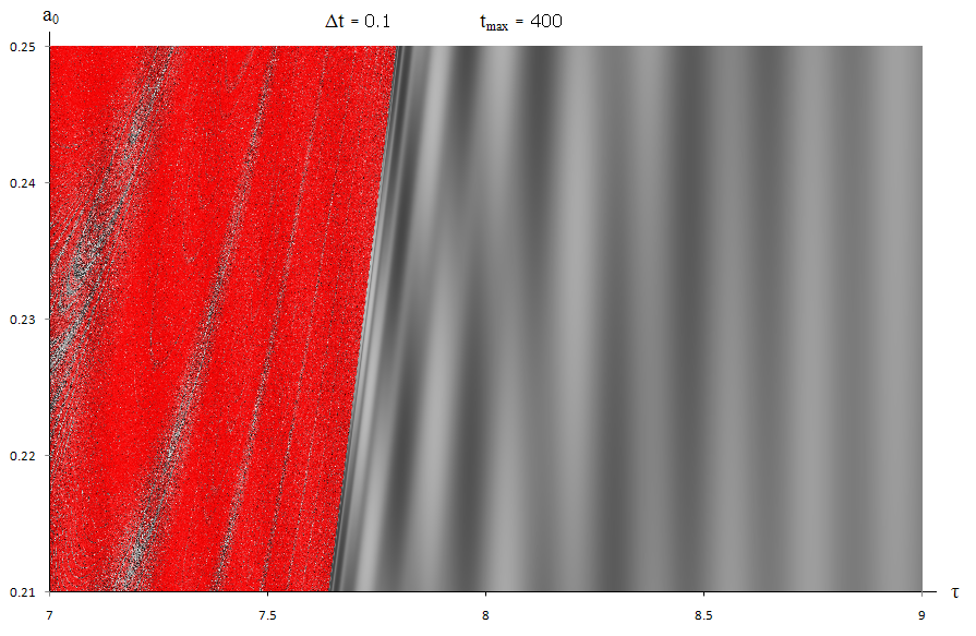
Figure 7.
Values of θ for 0.21 < a₀ < 0.25 and 7 < τ < 9 with t_max = 400
A deeper hue means θ spent a bigger fraction of the simulation outside the region ( -π , π )

As time evolves, the chaotic regions become clearer and spread asymptotically. The red highlight follows the same area exactly, as can be seen by comparing Figures 2&3 to Figures 6&7. Zooming out, the boundary of chaos surrounds the regular, predictable pattern in a parabola (Figure8). Outside this region the pendulum behaves like a single pendulum as the amplitude of M is too small, or the period of M is too large, to have an effect. The base of the region marks the resonant frequency of the lower pendulum (ref3).

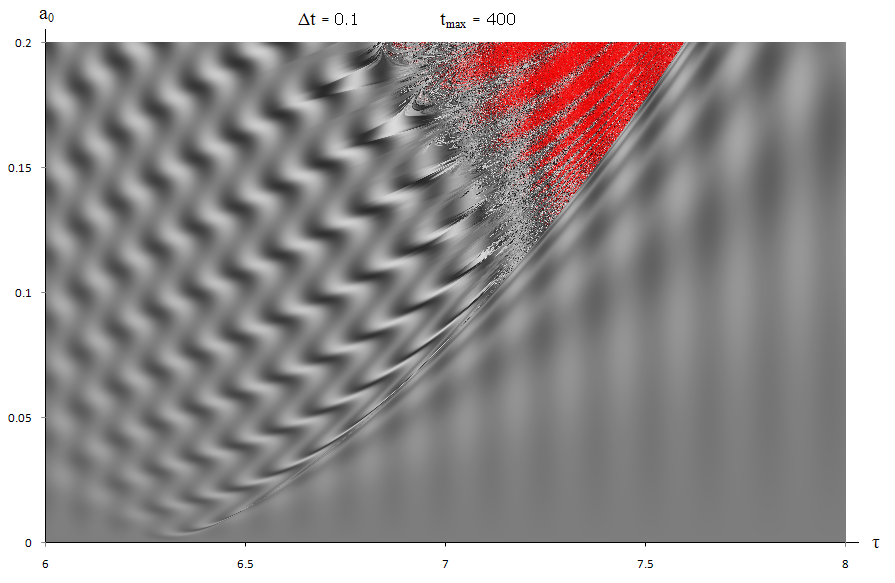
Figure 8.
Values of θ for 0.0 < a₀ < 0.2 and 6 < τ < 8 with t_max = 400 The chaotic region draws out a parabola over time.

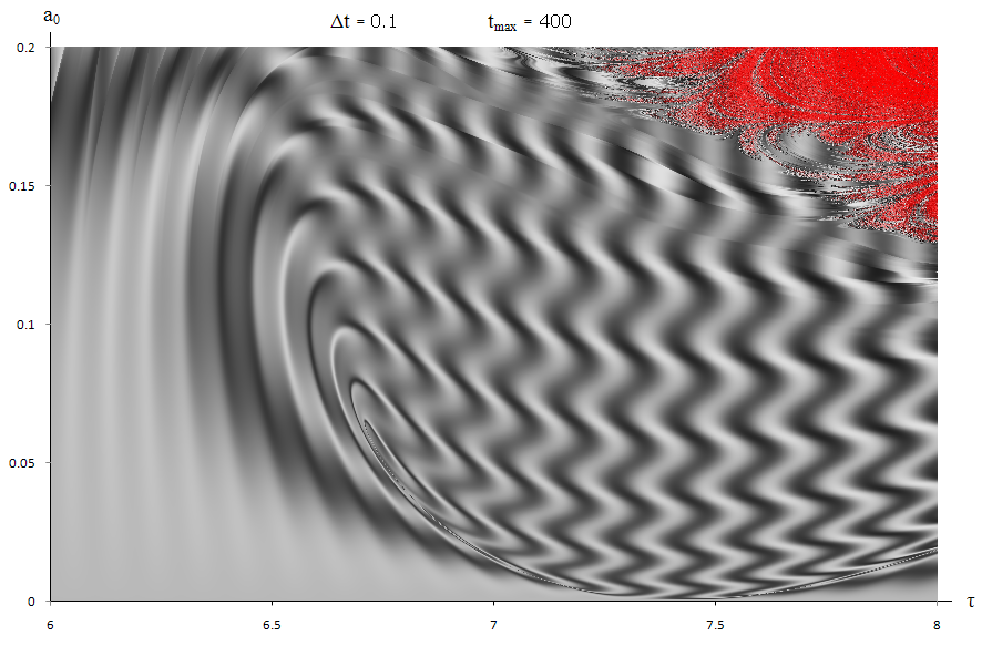
Figure 9.
Same as figure 8 but with θ_init=π/2

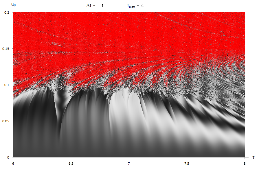
Figure 10.
Same as figure 8 but with θ_init=3π/4

Investigating the dependency on initial conditions, Figures 9&10 show how the same area changes when Equation and (ω_init is kept constant). The chaotic region grows as the pendulum can escape the normal region much easier. At the graph becomes pure chaos. Changing ω_init would produce similar (but skewed) graphs, akin to jumping ahead in the simulation.

Choosing levels of accuracy is a compromise with computing power and available time. Reducing Δt makes the regions clearer but takes longer to render. Throughout the simulations Δt=0.1, chosen after examining Figure12.

Throughout, all decimal variables were stored as double floats (8 bytes). This gives around 16 places of precision. The limitations of the program are visible when simulations are made in steps of ~10^-17 (Figure11). When investigating chaos, rounding errors can have a huge effect on the output (ref2). However, the graphs in this simulation were plotted in steps of ~10^-5 hence rounding errors should not have effected the results significantly.

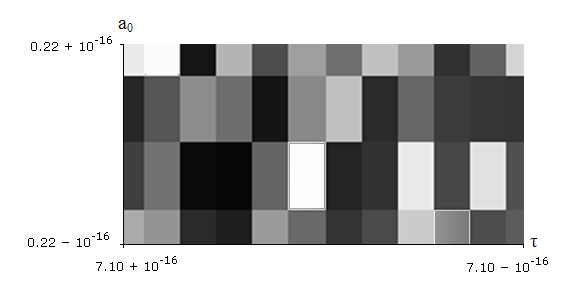
Plot of the extremes of the floating point resolution

Figure 11.
Extremely high resolution plots become “pixilated” as the limitations of variable accuracy become evident.

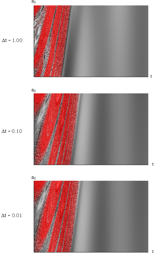
Figure 12.
Three test plots of the same area for different values of Δt. The upper and centre plots show noticeable differences, whereas the lower and centre plots have negligible difference, justifying the use of Δt=0.1 as a compromise.

The model itself is only an approximation, assuming the angle of M remains small. This has shown the basic concepts of a double pendulum but a more relevant result would be achieved if m ≈ M. A plot of initial angles for both pendulums on either axis would produce a result similar to Figure13.

Figure 13.
Double Pendulum plot by Jeremy S. Heyl
The colour of each pixel indicates whether either pendulum of a double pendulum flips within 10 (green), within 100 (red), 1000 (purple) or 10000 (blue). Those that don't flip within 10000 are plotted white. The angle that the upper pendulum makes with the vertical initially ranges from -3 at the left-hand side of the plot to +3 at the right-hand side. The angle that the lower pendulum initial makes with the vertical ranges from -3 at the top to +3 at the bottom.

References

David Clements, First Year Computing Laboratory, Version 2.9
Raymond Sneyers (1997) "Climate Chaotic Instability: Statistical Determination and Theoretical Background", Environmetrics, vol. 8, no. 5, pages 517–532.
Meirovitch, Leonard (1986). Elements of Vibration Analysis (2nd edition ed.). McGraw-Hill Science/Engineering/Math.

Appendix A: C++ Source code for the main simulation & modification 1 

#include <iostream>                     // Include headers for i/o,
#include <fstream>                      // file writing,

#include <cmath>                        // and mathematical functions
using namespace std;
double doublePendulum(double, double);  // Prototype for our simulation

const double pi = 2*acos(0.0);          // Define pi
double tmax,dt,toutside;                /* Declare variables tmax, dt, and
                                           toutside which need to be global */

int main() 
{
    /*  First we need to create the image we will be plotting to.
        We achieve this by reading the header data from a blank
        bitmap file and storing in the variable str[]. 
        The width and height of the image are also read, in order
        to set the resolution of our graph plot.
    */
    char str[54];    //Header data for a bitmap is 54 bytes


    // Open file in binary read mode and read the first 54 bytes
    ifstream blankfile("blank.bmp",ios::in | ios::binary);

    blankfile.read(str,54);

    unsigned int width,height;

    blankfile.seekg(18);                // Read WxH from header data
    blankfile.read((char*)&width, 4);   // which are unsigned integers

    blankfile.read((char*)&height, 4);  // at positions 18 and 22

    double a0min,a0max,taumin,taumax,theta; //Input data from user

    cout << "Double Pendulum plot. Enter initial conditions.\na0 min:\n";
    cin>>a0min;
    cout << "a0 max:\n"; cin>>a0max;

    cout << "tau min:\n"; cin>>taumin;
    cout << "tau max:\n"; cin>>taumax;

    cout << "t max:\n"; cin>>tmax;
    cout << "dt:\n"; cin>>dt;

    
    /*  We now have enough information to create the new file. 
        For convienience, the values used will be stored in the filename.
        We construct this filename using the sprintf() function, which
        can combine numerical variables as a string. */
    char filename[255]; 
    sprintf(filename, "output5/p%f_%f_%f_%f_%f_%f.bmp", 
                        a0min,a0max,taumin,taumax,tmax,dt);

    
    // Open the file for writing in binary mode
    ofstream myfile(filename,ios::out | ios::binary);

    // Write the 54 byte header we read earlier
    myfile.write(str,54);
    
    /*  Next is the main cycle which plots every pixel on the graph.
        The nested loops travel through each x and y value (i and j)
        and the subroutine doublePendulum() is called. Values of a
        and tau are calculated based on the limits provided earlier
        by the user. 
    */
    char rgb[3]; // 3 bytes per pixel


    for (int j=0;j<height;j++)            // Vertical loop (rows)

    {
        for (int i=0;i<width;i++)         // Horizontal loop (columns)

        {
            //Call the function with the values from the loop 
            theta = doublePendulum( a0min + j/(height/(a0max-a0min)),

                                    taumin + i/(width/(taumax-taumin)));


            /*  The pixel brightness is determined by theta.
                We need to scale theta from the range -pi, pi into 0, 255
            */

            rgb[0]= 127*theta/pi;
            
            /*  Colour Adjustment. Saturation is determined by the difference
            between the pixel values - three identical values gives a gray
            pixel. To highight areas where the pendulum has left the range of 
            -pi, pi we take the fraction of time outside, and multiply it by 
            the difference between the current pixel value ( rgb[0] ) and 255.
            This value is added to the red pixels ( rgb[2] ) and subtracted 
            from the green and blue.
            */
            rgb[2]=(rgb[0]+(127-rgb[0])*toutside/tmax) + 127;

            rgb[1]=(rgb[0]-(127+rgb[0])*toutside/tmax) + 127;

            rgb[0]=(rgb[0]-(127+rgb[0])*toutside/tmax) + 127;

            
            // Write this pixel to the file
            myfile.write(rgb,3);
        }

        // Loading bar - clear screen and calculate percentage

        system("CLS");
        cout << "Rendering . . . " << 100*j/height << "%";

    }
    /*  Launch our image for viewing.
        The file must be closed, and then a system call can be made to open
        the image. For convienience, the filename variable is reused to 
        construct the command.
    */
    myfile.close();
    sprintf(filename, "cd output5 & p%f_%f_%f_%f_%f_%f.bmp", 
                                    a0min,a0max,taumin,taumax,tmax,dt);

    system(filename);
}

// Actual pendulum simulation routine
double doublePendulum(double a, double tau) 

{
    // Declare variables
    double omega=0.0,theta=0.1,t=0.0;

    toutside=0;

    // Begin simulation loop
    while (t < tmax) 
    {

        /*  In each step of the simulation, t increases by dt, and so theta 
            and omega are increased by their calculated values multiplied by dt.
        */
        t+=dt;
        theta+=omega *dt;

        omega-=dt*(sin(theta) + a*sin(2*pi*t/tau)*cos(theta));

        /*  We record the time the pendulum spends outside the normal
            region in the variable toutside. This should have a direct
            correlation to the chaotic regions.
        */
        toutside+=(theta>pi | theta<-pi ? dt:0);

    } 
    return theta;
}





Appendix B: Source code for phase-space plots

#include <fstream>                  // Include headers for file writing
#include <cmath>                    // and mathematical funtions

const double pi = 2*acos(0.0);      // Define pi


int main() {                        // Declare variables and initial values
    double omega=0.0,theta=0.1,t=0.0,dt=0.1,a=0.251,tau=8,tmax=100;

    std::ofstream myfile("phase-space/out.txt"); //Open file for writing

    while (t < tmax) {              // Begin simulation

        t+=dt;                      // Iterate values - same as simulation 1, 
        theta+=omega *dt;           // see main text for formulae

        omega-=dt*(sin(theta) + a*sin(2*pi*t/tau)*cos(theta));

        myfile << theta << "\t" << omega << "\n"; // Write output to file

    } 
}

The output in this file was then fed into and plotted using MS Excel.