
Faster than a FFT
3 Oct 2014Progress: Completed
You guessed it, it's another Reverse Oscilloscope side-project. A continuation of my investigations into anti-aliased sound generation.
Motivation
As we know, the synthesizer has to resample the waveforms you've drawn to be at the correct pitch. In the same way that if you resize an image by an odd amount, you get aliasing (nearest-neighbour, like in MSPaint) unless you make some kind of correction for it (eg bicubic, like photoshop).If you're not yet convinced of the need to do this, consider the sound generation of a simple square wave. The sound card sends samples to the speaker at, for instance, 44.1kHz. We could send five samples of -1, then five samples of +1, and repeat, and this would give a perfect square wave. The period of ten samples would give a pitch of 4.41kHz. Sending four samples of -1 and four of +1 would give a pitch of about 5.5Hz. So what if we want a pitch in between 4.4kHz and 5.5kHz?
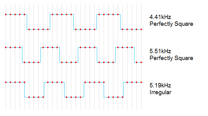
The fact is, you just can't do it. There is no way of making a perfect square wave that doesn't line up to the 'grid' of the samplerate. The third wave above lines up with samples for lengths of 5, 4, 4, 4, 5, 4, 4, 4 and so on. Not only is this not a perfect square, but there's a new frequency introduced - the pattern repeats every two periods. This lower frequency can be heard, and is called aliasing.
The phenomenon is well known and takes many forms in many different fields. In digital sampling, we say that you cannot generate a frequency higher than half the samplerate, called the Nyquist frequency. That'd be one +1, one -1, etc. or a period of two samples. Seems simple enough, but it takes some thinking to realize that this applies to waves of much lower frequencies. In essence, a perfect square wave has infinite bandwidth, meaning its frequency components go up to infinity, and so by definition we have gone above the Nyquist frequency. The result is that these higher frequencies wrap around into the lower ones and become aliasing.
But our ears can only hear up to, at most, 20kHz, so generating higher frequencies is pointless. A square wave with the higher components cut out looks like this, and sounds exactly the same:
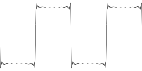
The wiggly bits are normally called the Gibbs phenomenon, but here, we're adding them in on purpose so as to directly counteract the aliasing. And it works. But generating a bandlimited wave like this isn't easy, as those wiggles are specific to that particular wave, at a particular frequency, at a particular samplerate. This is a very difficult calculation.
Update: there was originally a paragraph here which was incorrect. Someone described to me how square waves can be generated by pre-calculating the transitions, and I misunderstood it to be how old consoles like the Gameboy generated sounds. They of course had dedicated hardware to produce square waves. The "band-limited step" approach to generating square and sawtooth waves is really interesting and you should look it up.
But in case you hadn't noticed, for the Reverse Oscilloscope we need more than square waves.
Working with a spectrum
The synthesizer has dealt with the time and frequency domains equally for a while now, but even my best anti-aliasing attempts have only been working in the time domain. It's common sense to make a time-domain signal from a time-domain waveform, but for the ultimate in aliasing-reduction I had tried to transform into fourier space, clip the spectrum, and transform back. The obvious thing to do then is skip the first transform and try and generate the sound completely from the original waveform's spectrum. In a way, we're ignoring the oscilloscope part of the reverse oscilloscope completely.It is, however, quite computationally expensive to perform a fourier transform for every note. Additionally, I'm not entirely sure how you go about doing this using an unmodified FFT algorithm, given that we have to resample to use a basis that isn't a power of 2.
Let's get to the point. About three months ago I came up with a method of generating a time domain signal, at the correct pitch, from an arbitrary frequency spectrum, fast enough to be used in real time with my synthesizer. It only really works with music synthesis, because by its nature it isn't as accurate as a real inverse FFT: phase data progressively drifts all over the place, but this is completely inaudible.
You might want to go get a cup of tea at this point.
Here's a triangle wave from the interface of the synthesizer:
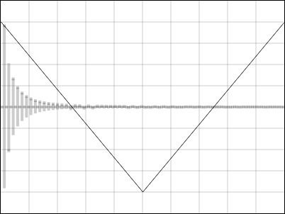
The grey rectangles along the middle are a bar graph of its Fourier components. Every other component is zero - a feature of triangles and squares. What this means is to generate this wave at, for instance, 100Hz, we would need a large amplitude sine wave at 100Hz, nothing at 200Hz, a lower amplitude sine wave at 300Hz, nothing at 400Hz, an even lower sine at 500Hz, nothing at 600Hz, and so on. We add all these up and we get a lovely triangle, or even with the wrong phase, something that sounds identical to a triangle. This process is called an Inverse Fourier Transform. If the Nyquist frequency were at 1000Hz, we would simply stop adding sine waves when we get to that point, and we're left with a perfectly bandlimited triangle.
It is possible to do just this, which works, but is hugely expensive processor-wise. Remember that a sine call is a very slow operation, compared to, say, multiplication. We have to do, what, 512 sine calls per sample? Or more? So in comes the Fast Fourier Transform. It's fast all right, but as I've mentioned, it's not fast enough. Additionally, the normal FFT (the butterfly algorithm thing) requires a power-of-two fundamental period. It is possible, presumably, to track all the phase data correctly and work with this. I couldn't manage it however. Resampling isn't feasible; it's slow and may introduce even more aliasing.
From the title of this project you'll have guessed there's a better way of doing this. We're still not there yet though. Another digression before I can start to explain my algorithm...
One line filters
I've had an obsession with them since I discovered them - well, since I first saw the filter algorithm in a DSP library that offered Lowpass, Highpass, Bandpass and Bandstop, with adjustable resonance and cutoff, and did this in four lines of code. Not even micro-optimised.It was what you'd call a two-pole, or biquad, Infinite Impulse Response filter. For someone like me, with absolutely no background in signal processing, this was gobbledygook. Filter design is a massive field, but even after researching it, and getting my head around complex contours, zeros and poles, Laplace transforms and transfer functions, I still hadn't answered the main question: how was this feature-rich function so mathematically concise?
Most of the information you'll find on this is, naturally, about how to design filters. That's why they're working in the Laplace domain, it pads it out into something you can visualise. The algorithm of the filter itself is just a single equation that takes a sample, mangles it and spits it out.
Looking at the very simplest of filters though, it is possible to understand it after all. Let's take a one-pole lowpass IIR filter.
output = ( state_variable += fraction * (input - state_variable) )If you've played with my visual demonstration of filters you should know how it responds to a simple step function. Instead of jumping to the input value, it moves only a percentage of the way there. In fact, this is the same equation I've used to simulate portamento, or to smooth the slider motion. In fact, it's the same equation that we used to use to smooth the viewport motion at Kousou Games. The smooth tracking of the player in tLoZ:The Final Challenge, was, in fact, a single-pole lowpass IIR filter. Put simply, the output exponentially approaches the input value.
A one-pole filter requires one state variable (that's kept in memory from one sample to the next). I suppose you could say that a waveshaper, with a one-to-one map between input and output, is like a zero-pole filter. Maybe.
The fraction corresponds (~inversely) to the cutoff frequency. We can also make a highpass filter, cleverly, by subtracting this lowpass value from the input. Confident of our understanding here, next, a two-pole filter is like two filters combined. If they were identical, we would get a lowpass filter with twice the rolloff. If one were highpass and one were lowpass, they could be combined to give a notch or a bandpass. Finally, by feeding a fraction of the input back into the filter, we can simulate resonance.
I picture this in my mind as two Bode plots being smooshed together, but I suppose that's no better than imagining the tent-poles of complex space being dragged towards a contour integral. Having said that, I think that the above paragraphs, combined with some algebraic rearrangement, is the best we will ever get to understanding that magical biquad filter.
(In no do I way mean to detract from the 'official' explanation. If you want to know more about filter poles, this is the most concise, simple, informative introduction to the field I've been able to find, and I dearly wish that I had found it sooner.)
Self-oscillation
When we want a sine wave, we usually make continuous calls to the sine() function, every sample. But this inherently feels wasteful, since each call is asking for a fixed increase in phase, but it's calculating or looking it up from scratch.So a thought occurred to me. If the resonance of a filter is turned to maximum it goes into self-oscillation. Then, it's outputting a pretty accurate sine wave, even though each sample is only generated through an arithmetic combination of the previous two. We won't be able to jump to a known phase, but in audio synthesis, we don't need to. The only trigonometric call we need to make is at the beginning, to calculate the coefficient (fraction).
The equation then is just:
output = fraction * s1 - s2;
s2 = s1;
s1 = output;
where the fraction, which determines the frequency, is calculated from a single cosine call. The output is a sinewave with just one multiplication and one subtraction per sample.
So that was the basic idea for our inverse fourier transform: a massively parallel bank of self-oscillating IIR filters. We need to track every one of them, and remember all their state variables, but that's no trouble. However we're still faced with a problem if we want to change (or when we initially decide on) the frequency. That means possibly hundreds of trigonometric calls at once - but here's the clever bit. The frequencies are all multiples of the fundamental. That means the coefficients themselves form a trigonometric progression. That means we can calculate them, too, using a self-oscillating IIR filter. The end result is an inverse transform which only makes one single trigonometric call.
Obviously it isn't the most accurate, with all those multiplications the floating point errors soon add up and the phase starts to drift, but it's recalculated from scratch at the beginning of each envelope, so we needn't worry.
Is it faster than an FFT? It's not really a fair comparison to make, because the targets are different.
Is this method of additive synthesis faster overall than trying to use a FFT to bandlimit the normal method of wave generation? Yes.
Is it faster than what I was doing before? Sort-of. Not really. Only if you sacrifice the upper frequencies of the lowest notes.
So far I've only implemented a single-waveform version, but the interpolation should not be difficult to add. The number of partials that it uses is of course related to the fundamental frequency and the Nyquist frequency, so the lower the note you play, the harder it has to work. This is the exact opposite of the FIR smoothing the scope currently performs, which works harder at higher pitches. So I think the next thing to do is to combine the old and the new algorithms: time-domain generation for the low notes, frequency-domain generation for the high. Although I've yet to implement it, this promises an ideal combination of alias-free sound with a low computational power requirement.
Or perhaps I should make a toggle to switch between algorithms. After all, phase data is vitally important when you're using waveshapers. Additionally the aliasing tends to get drowned out when you're dealing with distortion synthesis.
I'm quite proud of this creation actually. It's one of those ideas that comes to you all of a sudden, but you're too busy to implement it. Then when it comes to building it you doubt if it actually would work. And then you find it works perfectly first time, and you smile.
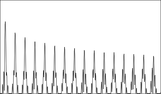
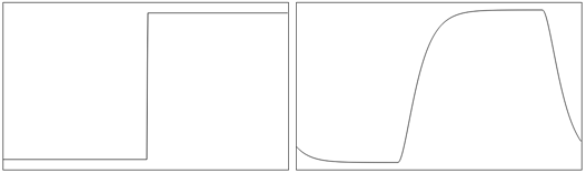
The hideously aliased spectrum of a naively resampled square wave
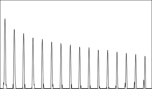
A fairly good compromise by my most recent time-domain algorithm
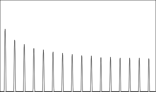
Perfection at the hands of my self-oscillating filter bank
Addendum
I wrote the algorithm described above several months ago. After posting this projects page (enthusiasm renewed) I went back and finished it, adding the interpolation in, and crucially, merging the code with the scope properly instead of just pasting it into the console. That makes it run a lot faster.Having played with them side-by-side, I'd say the two algorithms are about equal in terms of speed in the normal range of notes. As you get very high, the old algorithm struggles; as you get very low, the new one starts to choke. I'm not sure if I'll make a hybrid version, but the next release of the synth has a dropdown box to choose which one you want to use. I'll write some more on the main Reverse Oscilloscope page.